Guided Workflow: GBT Burst
This walkthrough follows a single GBT-L burst from loading through preparation, measurements, width comparison, DM optimization, temporal diagnostics, fitting, and export.
The example file is a SIGPROC filterbank from DIAG_FRB20240114A:
blc_s_guppi_60385_53711_DIAG_FRB20240114A_0057_1673.964_1675.753_b32_I0_D527_851_F256D_K_t30_d1.fil
The filename records D527_851, but this cutout is already dedispersed. Load it
with DM = 0 in FLITS. Use the DM tab later only as a local residual/refinement
diagnostic around zero.
1. Download the tutorial burst
mkdir -p tutorial-data
curl -L -o tutorial-data/flits-tutorial-gbt-frb20240114a-v1.fil \
  https://github.com/DirkKuiper/flits/releases/download/tutorial-data-v1/flits-tutorial-gbt-frb20240114a-v1.fil
For development checkouts that already have the ignored local data directory, the source file is:
data/GBT-L/blc_s_guppi_60385_53711_DIAG_FRB20240114A_0057_1673.964_1675.753_b32_I0_D527_851_F256D_K_t30_d1.fil
2. Start FLITS
Open http://127.0.0.1:8123.
In the loader:
- Select
flits-tutorial-gbt-frb20240114a-v1.fil. - Enter
0for DM. - Leave the preset on the detected
GBTsetting. - Load the session.
Expected first-session checks:
256channels- full time span of about
423 ms - native sample time of
10.24 us - default plotted time bins reduced by
x32, or327.68 us - GBT calibration preset with
10 JySEFD - the bright burst is near
240 ms
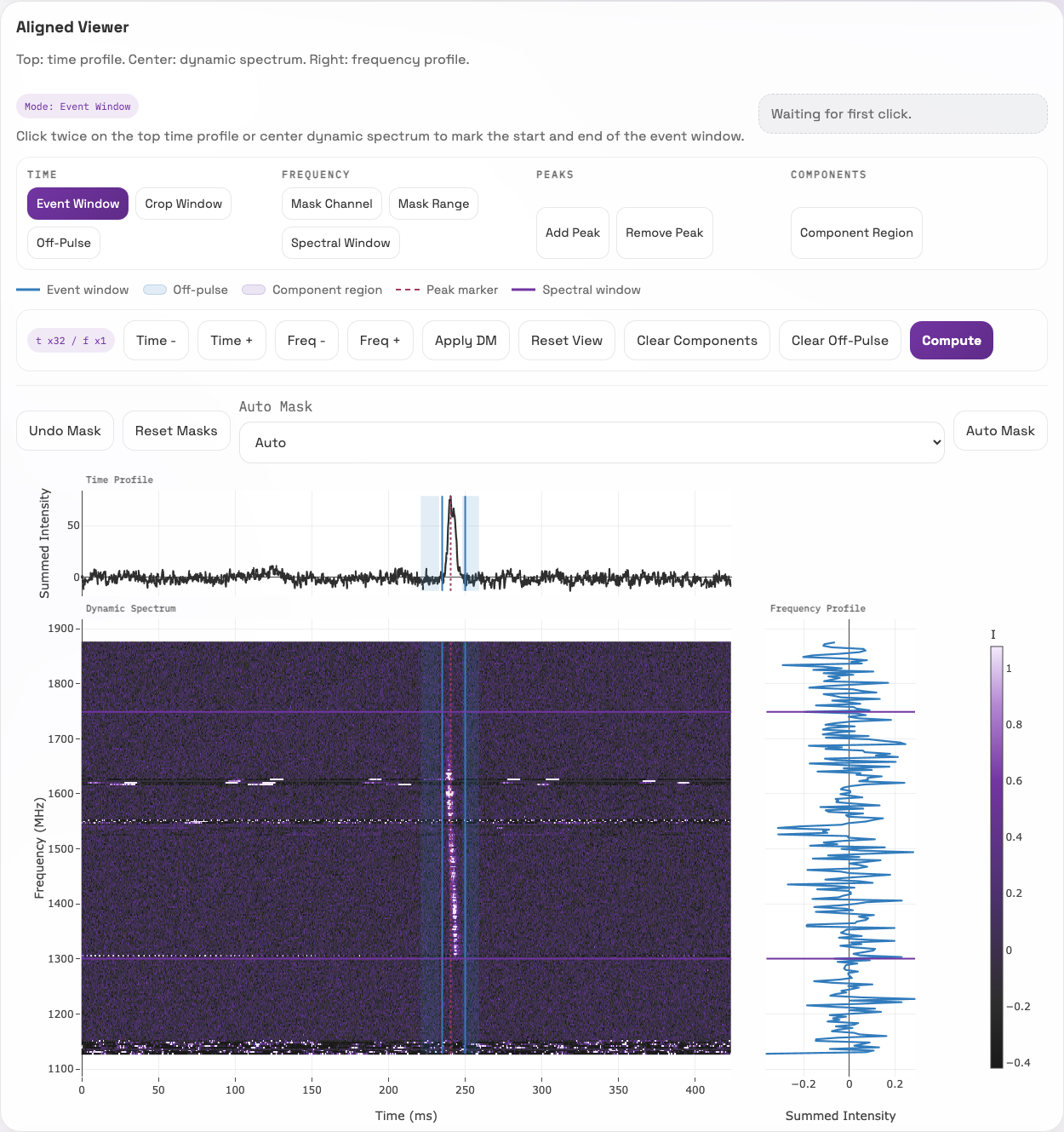
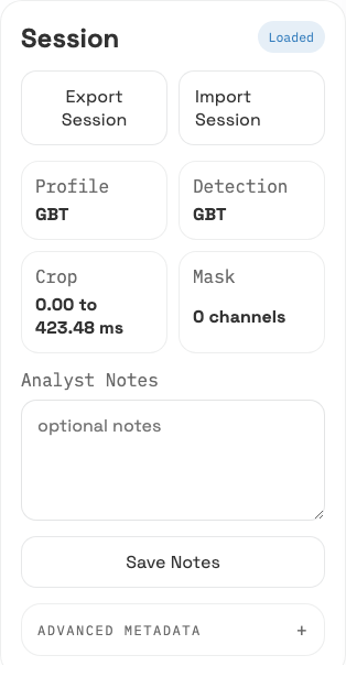
3. Prepare the burst
Use the Prepare controls to focus the analysis state before interpreting any numbers.
Set:
- event window:
235to250 ms - off-pulse windows:
221to233 ms, and248to259 ms - spectral window:
1300to1750 MHz - masks: optionally click 'Auto Mask' once
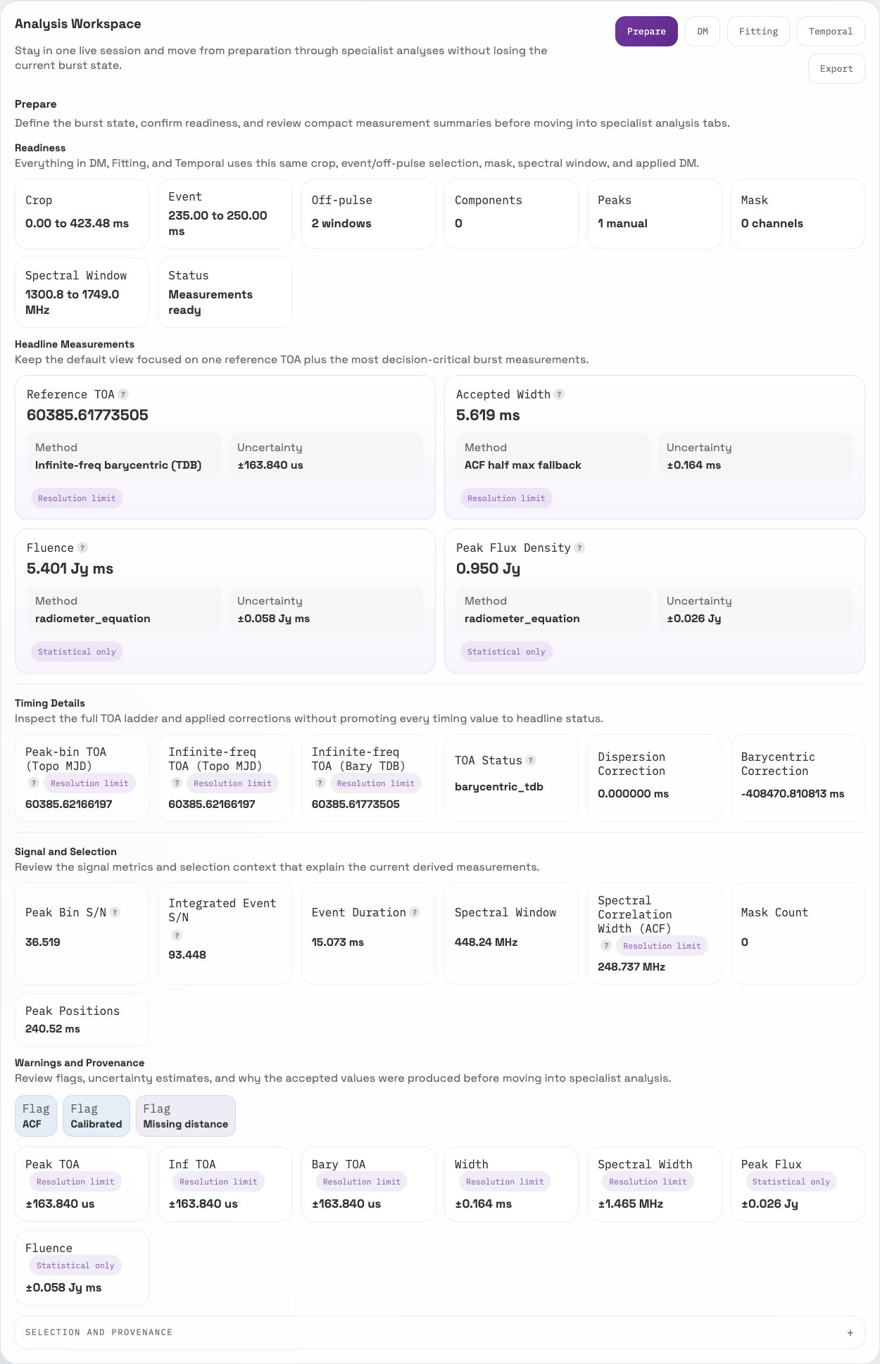
4. Compute measurements
Click Compute after the event, off-pulse, and spectral windows are set.
The exact values can shift slightly with selection quantization, but the result should be close to:
| Quantity | Expected value |
|---|---|
| Peak S/N | ~36.5 |
| Integrated event S/N | ~93.4 |
| Fluence | ~5.4 Jy ms |
| Peak flux density | ~0.95 Jy |
| Peak topocentric TOA | ~60385.62166196854 MJD |
| Infinite-frequency topocentric TOA | ~60385.62166196854 MJD |
| Barycentric TDB TOA | ~60385.61773505590 MJD |
Because the session DM is 0, the infinite-frequency correction is 0 ms and
the peak and infinite-frequency topocentric TOAs are the same. The expected
measurement flags are calibrated, acf, and missing_distance; the distance
flag is normal unless you provide a distance or redshift.
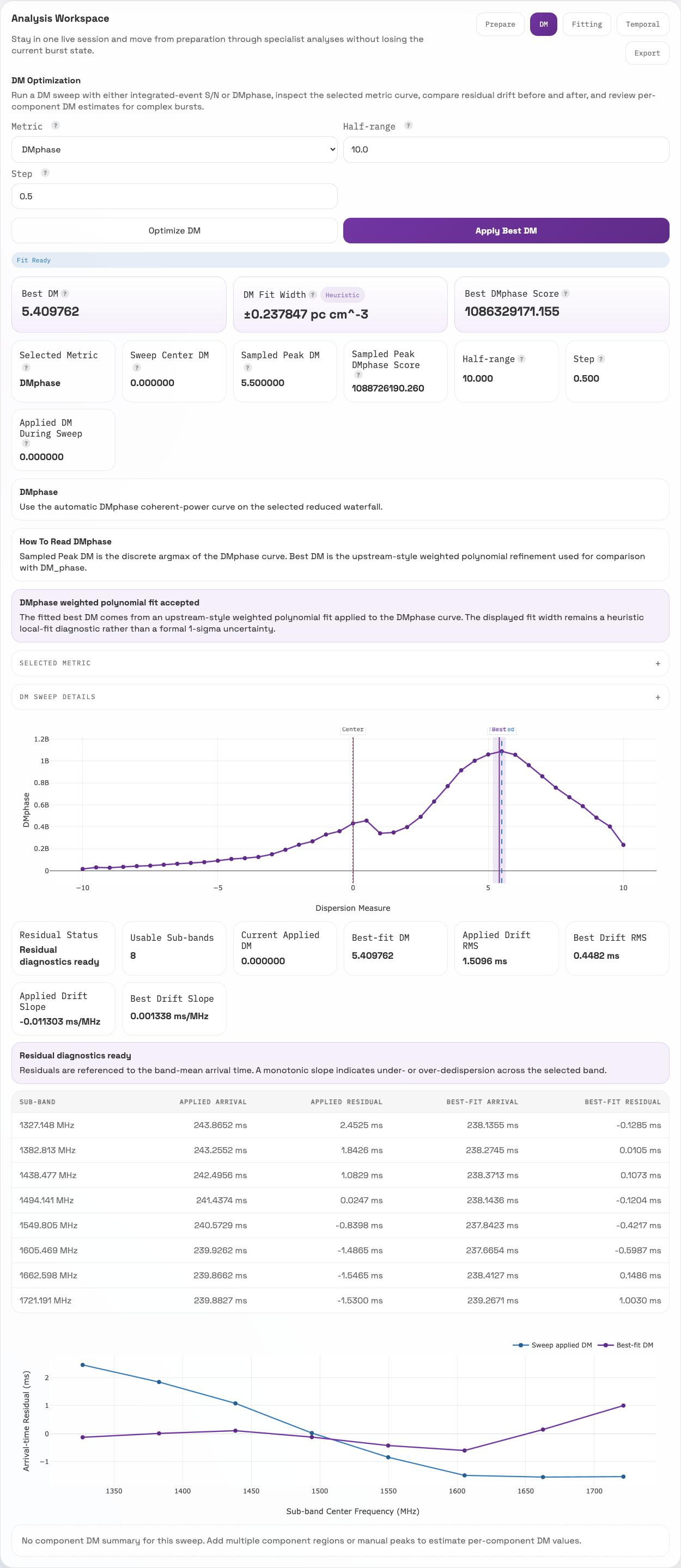
5. Run a local DM sweep
Open the DM tab and run a DMphase sweep with:
- center DM:
0 - half range:
10.0 - step:
0.5 - metric:
DMphase
Expected checks:
- best DM near
5.41 pc cm^-3 - sampled best DM near
5.5 pc cm^-3 - fit status:
dmphase_weighted_polyfit - residual status:
ok
6. Export the session for reproducibility
Use Save Session in the sidebar after the event window, off-pulse windows, spectral window, mask state, measurements, and DM sweep are where you want them.
The saved JSON snapshot stores the interactive session state, not just the final
values. FLITS writes it into a snapshots/ folder next to the source data so the
analysis can be reopened later from Saved Sessions and inspected from the
same crop, selection, masking, calibration, notes, and analysis state. Use
Download JSON only when you need a portable copy outside the snapshot
library.