Temporal and Spectral Analysis
These diagnostics all run on the event profile: the dynamic spectrum summed over the current spectral window and restricted to the current event window, with masked channels excluded. Changing the mask, the spectral window or the event window changes every result on this page.
What is computed
| Diagnostic | Question it answers |
|---|---|
| Autocorrelation (ACF) | On what timescale does the profile resemble a shifted copy of itself? |
| Raw periodogram | How is variance distributed over fluctuation frequency, unaveraged? |
| Averaged PSD | The same, with segments averaged to reduce variance. |
| Minimum-structure scale scan | What is the finest structure that is statistically significant in this burst? |
| Power-law plus constant PSD fit | Does the variability follow a power law, and where does it meet the noise floor? |
| Crossover frequency | The fluctuation frequency where the fitted power law meets the constant term. |
Choosing a segment length
Segment length is the main control, and it is a direct trade-off. The event window of length \( T \) split into segments of length \( T_\mathrm{seg} \) gives frequency resolution \( \Delta f = 1/T_\mathrm{seg} \) and roughly \( T / T_\mathrm{seg} \) independent averages.
- Longer segments: finer frequency resolution, noisier estimate at each frequency.
- Shorter segments: smoother, more reliable PSD, but coarser in frequency and blind to fluctuations slower than one segment.
There is no universally correct choice — it depends on the event length and the
timescales you care about. default_segment_bins picks a conservative default
from the event length; override it when you have a specific timescale in mind.
A practical check: if the PSD changes character substantially when you halve the segment length, the feature you are looking at is not yet well constrained.
Interpreting the scale scan
The minimum-structure scan reports the smallest structure that is statistically significant in the current profile. Two cautions:
- It is not the burst duration, and not a physical timescale of the source. It is a detection threshold, so it depends on signal-to-noise. A brighter observation of the same burst will report finer structure.
- If the response is still rising at the largest tested scale, that means either broad emission or no turnover inside the tested range — not that the burst has no characteristic scale.
For comparing bursts of unequal brightness, use the noise-subtracted multiscale estimator instead, which is built to remove exactly this S/N dependence.
ACF widths are not durations
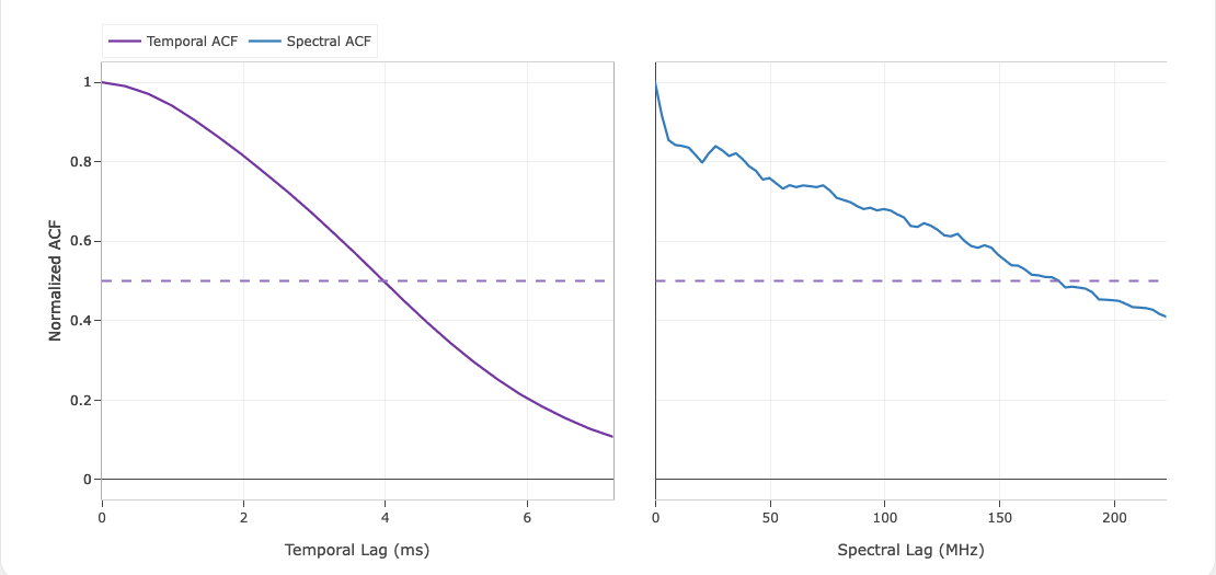
The dashed line marks normalized ACF = 0.5. Its intersections with the curves give self-similarity widths in time and frequency for the GBT example, not the manually selected event duration.
An ACF width is a self-similarity scale. It is a good way to compare coherence structure between bursts or between time and frequency, but it is not interchangeable with the full burst duration, and the two can differ by a large factor for a multi-component burst. Report which one you mean.
The PSD fit is deliberately simple
The model is a power law plus a constant:
with \( C \) representing the white-noise floor. This is enough to characterise whether variability is scale-free over the fitted range and where it disappears into the noise. It is not a physical model of the emission.
When the fit is poorly constrained — a short event, low S/N, or a PSD with curvature the model cannot represent — the stored fit status matters more than the nominal parameter values. FLITS records that status alongside the parameters precisely so a spectral index is not quoted from a fit that did not converge. Check it before using \( \alpha \) for anything.
The crossover frequency is reported only when the fit is well enough constrained for it to mean something.
Practical sequence
- Mask interference and set the spectral window before running anything here — every diagnostic is computed on what those leave behind.
- Set the event window to the burst, and the off-pulse regions to genuinely burst-free data used as the noise reference.
- Start with the default segment length, then vary it to check stability.
- Read the fit status before the fit parameters.
- For population work, prefer the multiscale estimator and calibrate with injections.