DM Optimization
FLITS sweeps trial DMs around the current value, scores each one, and reports the DM that maximizes the chosen criterion. Two criteria are available, and they answer different questions.
How dedispersion works here
FLITS dedisperses incoherently to the top of the band. The delay of a channel at frequency \( \nu \) relative to the reference frequency \( \nu_\mathrm{ref} \) (the highest channel) is
using the pulsar-astronomy convention for \( k_\mathrm{DM} \) rather than the exact physical constant — see References.
Each channel is shifted by a whole number of samples. Two consequences follow, and both matter when choosing sweep parameters.
The DM resolution is set by the time resolution
Because shifts are rounded, there is a smallest DM step that moves anything at all: the step that shifts the lowest channel by one sample,
Trials spaced more finely than this are bit-identical. A sweep stepped below it wastes work and produces a score curve that looks smooth because neighbouring points are the same data, not because the metric is well behaved.
flits.signal.dedispersion_bin_resolution computes this for a given band and
sampling. Use it to pick a step rather than guessing:
from flits.signal import dedispersion_bin_resolution

step = dedispersion_bin_resolution(session.freqs, session.tsamp)
session.optimize_dm(session.dm, half_range=2.0, step=step)
Results are tagged with an integer_bin_dedispersion warning flag as a
reminder that the reported DM cannot be more precise than this.
The window edges are not valid data
Samples shifted in from beyond the read window are not burst data. FLITS
zero-fills them when a file is loaded, rather than wrapping them around the time
axis where they would contaminate the off-pulse region. The affected extent is
reported by flits.signal.dedispersion_edge_bins. Keep the event and off-pulse
windows away from it; burst localization raises event_near_edge when the burst
sits too close.
The two metrics
Integrated-event S/N
Sums the dynamic spectrum over the spectral window to a profile, integrates the event window, and divides by the noise estimated from the off-pulse regions. The DM that maximizes this is the DM that makes the burst brightest and narrowest in the summed profile.
Use it when the burst is a single smooth component, and when signal-to-noise rather than structure is what you have to work with.
It is biased for bursts with downward frequency drift: a drifting burst is brightest when the drift is partly absorbed into the dispersion sweep, so the S/N-maximizing DM is systematically higher than the true one.
Structure maximization (DMphase)
A clean-room implementation of the DM_phase algorithm. Rather than maximizing brightness, it maximizes the coherence of the burst's Fourier phases across the band: at the correct DM, structure in different channels lines up in time, and the phases of the corresponding Fourier components agree.
Use it when the burst has sharp sub-structure, and whenever drift would bias the S/N metric. This is the criterion generally preferred for repeaters — see Hessels et al. (2019) in the References.
It needs structure to work with. On a smooth, low-S/N burst the phase coherence is weak and the score curve is correspondingly flat; the reported fit status will say so.
What the sweep depends on
The optimization runs against the current session state, not the raw file:
- the dynamic spectrum at the current DM
- the crop and event window
- the spectral window
- the channel mask
- the reduced-resolution (decimation) state
Changing any of them can change the preferred DM. This is a feature — masking a band of interference genuinely changes which DM best aligns what remains — but it means a reported DM is only meaningful alongside the state that produced it. That state is what the session snapshot records.
Reading the result
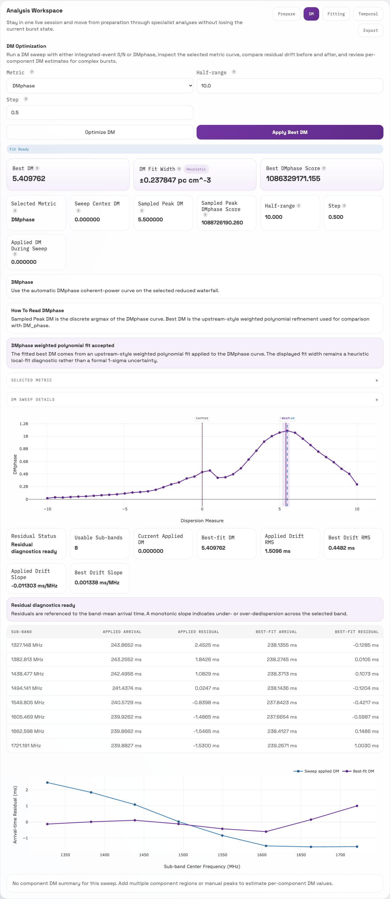
The DMphase curve peaks near a residual DM of 5.5 on the sampled grid; the weighted fit reports about 5.41. The lower plot compares sub-band arrival-time residuals at the applied and fitted DMs. See the GBT guided workflow for the inputs and interpretation limits of this example.
| Output | What to look at |
|---|---|
| Score curve | Should have a clear single maximum. Multiple comparable peaks mean the metric cannot distinguish them. |
| Preferred DM and fit status | A parabolic fit near the peak; peak_on_sweep_edge means the true optimum is outside the range you swept. |
| Residual arrival time | Structure remaining across the band after dedispersion, at both the applied and optimized DMs. |
| Warning flags | integer_bin_dedispersion always; others as they arise. |
Practical guidance
- Mask bad channels first — interference dominates the score otherwise.
- Restrict the spectral window to the part of the band you trust.
- Set a sensible event window; the S/N metric integrates exactly what you give it.
- Choose a step at or above the bin resolution above.
- If the peak sits at the edge of the sweep, widen the range and re-run.
- Pick the metric that suits the burst: structure maximization when there is structure or drift, integrated S/N when there is not.
- Treat the result as local to the analysis state, not as a context-free value.